UI Styling

The haskoning_equation package provides a comprehensive styling system for building consistent and interactive user interfaces. This includes styling for charts, tables, and individual form fields.

Overview

The styling system provides three main capabilities:

• CardStyle — Consistent card-like styling for components with titles, subtitles, and icons
• FieldStyle — Control UI rendering of individual form fields
• Component Styling — Material Design Icons (MDI) support and theming

CardStyle

CardStyle applies consistent card-like styling to chart or input components. It can be used at the field level or class level.

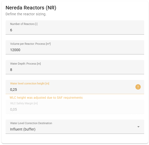
Split-layout: Field-Level Styling

This is the way to style a Split-layout application. An example is given here of a single panel in the UI. Field titles, descriptions and default values can be used to customize the way input fields are displayed. To style the panel itself, embed a CardStyle in a Pydantic field's json_schema_extra. Note the nesting of the basemodels in this example.

from enum import StrEnum
from pydantic import BaseModel, Field
from haskoning_equation.style import FloatFieldStyle
from haskoning_equation.units import units

class WlcDestination(StrEnum):
    INFLUENT = "Influent (buffer)"
    WLC_BUFFER = "WLC Buffer"
    EFFLUENT = "Effluent"
    OUT_OF_SCOPE = "Outside the Nereda-scope"

class NeredaReactorSizing(InputBaseModel):
    number_reactors: Annotated[int, Field(
        title="Number of Reactors",
        description="Number of reactors",
        ge=1,
        default=6,
        json_schema_extra={'unit': units.DIMENSIONLESS},
    )]
    reactor_volume: Annotated[float, Field(
        title="Volume per Reactor: Process",
        description="Process volume of a reactor. Possibly includes extra volume to "
        "accommodate the transition of DWF to RWF in case of CF without and IB.",
        ge=100,
        default=12000,
        json_schema_extra={'unit': units.VOLUME_STANDARD},
    )]
    water_depth_process: Annotated[float, Field(
        title="Water Depth: Process",
        description="Water depth when the reactor is aerating",
        ge=4.5,
        default=8.0,
        json_schema_extra={'unit': units.LENGTH_STANDARD},
    )]
    wlc_height: Annotated[float, Field(
        title="Water level correction height",
        description="Height for the water level correction (minimum value: 0.15 m)",
        default=0.15,
        ge=0.15,
        json_schema_extra={'unit': units.LENGTH_STANDARD},
    )]
    wlc_safety_margin: Annotated[float, Field(
        title="WLC Safety Margin",
        description="Safety margin for the water level correction",
        default=0.05,
        frozen=True,
        json_schema_extra={
            'unit': units.LENGTH_STANDARD,
            'style': FloatFieldStyle(disabled=True),
        },
    )]
    wlc_destination: Annotated[WlcDestination, Field(
        title="Water Level Correction Destination",
        description="Destination of WLC Discharge (if SAF it is backup WLC destination)",
        default=WlcDestination.INFLUENT,
    )]
    sludge_discharge_height_cache: Annotated[float, Field(
        default=0,
        json_schema_extra={
            'unit': units.LENGTH_STANDARD,
            'style': FloatFieldStyle(disabled=True, hidden=True)})]

class ProcessSetup(InputBaseModel):
    nereda_reactors_sizing: NeredaReactorSizing = Field(
        NeredaReactorSizing(),
        json_schema_extra={
            'style': CardStyle(
                title="Nereda Reactors (NR)",
                subtitle="Define the reactor sizing."
            )
        }
    )

This leads to the following UI panel:

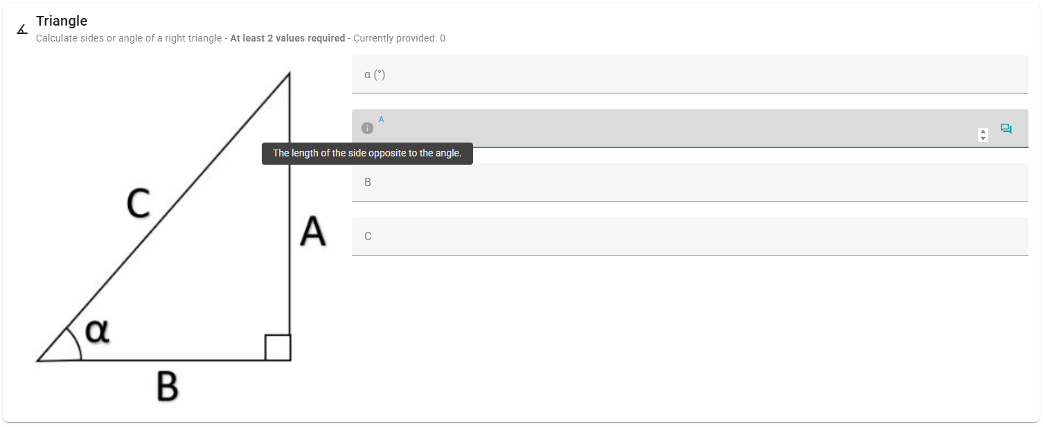
Combined-layout: Class-Level Styling

Use the way below to style a combined-layout application. Use the @apply_style decorator to attach a style to an entire model:

from pydantic import BaseModel, Field
from haskoning_equation.style import apply_style, CardStyle

@apply_style(
    style=CardStyle(
        title="Triangle",
        subtitle="Calculate sides or angle of a right triangle",
        icon="mdi-angle-acute",
        min_inputs=2,
        image_url="/haskoning_basic_hydraulics/static/images/driehoek.jpg",
    )
)
class TriangleInput(BaseModel):
    angle: float | None = Field(
        default=None, title="α (°)", description="The angle of the triangle in degrees."
    )
    opposite: float | None = Field(
        default=None, title="A", description="The length of the side opposite to the angle."
    )
    adjacent: float | None = Field(
        default=None,
        title="B",
        description="The length of the side adjacent to the angle.",
    )
    hypotenuse: float | None = Field(
        default=None, title="C", description="The length of the hypotenuse."
    )

    @model_validator(mode="after")
    def check_at_least_two(self) -> Self:
        check_minimum_number_of_inputs(self, 2)
        return self

The result of this in the ui is:

FieldStyle

FieldStyle classes control UI rendering of individual fields. Use them in json_schema_extra to specify control type, disabled state, or visibility.

Available FieldStyle Classes

Class	Field Type	UI Controls	Default	Example Usage
BooleanFieldStyle	bool	switch, select	switch	BooleanFieldStyle()
IntegerFieldStyle	int	slider, textfield	textfield	IntegerFieldStyle(type="slider")
FloatFieldStyle	float	slider, textfield	textfield	FloatFieldStyle(disabled=True)
StringFieldStyle	str	textfield, textarea	textfield	StringFieldStyle()
EnumFieldStyle	Enum	select	select	EnumFieldStyle()

All styles support disabled, hidden, cols, offset, and css options for additional UI control.

Example Usage

from typing import Annotated

from pydantic import Field
from haskoning_equation.models import InputBaseModel
from haskoning_equation.style import IntegerFieldStyle, FloatFieldStyle
from haskoning_equation.units import units

class ScenarioSettings(InputBaseModel):
    scenario_duration: Annotated[int, Field(
        title="Scenario duration",
        description="Total scenario duration",
        default=24 * 60,
        ge=0,
        json_schema_extra={
            'unit': units.TIME_PHASE,
            'style': IntegerFieldStyle(type="slider"),
        },
    )]
    general_load_factor: Annotated[float, Field(
        title="General load factor",
        description="Load factor for the design",
        default=1,
        ge=0,
        json_schema_extra={
            'unit': units.DIMENSIONLESS,
            'style': FloatFieldStyle(disabled=True),
        },
    )]

Working with Charts

ChartSchema

ChartSchema provides type-safe ChartJS configurations. Below are examples for common chart types.

Line Chart Example

import math
import random

from haskoning_equation.style.chartjs_pydantic import (
    ChartSchema, ChartType, ChartData, Dataset, ChartOptions,
    PluginsOptions, LegendOptions, PositionType, ScalesOptions, 
    AxisOptions, InteractionOptions, InteractionMode
)

def create_default_line_chart_data(num_minutes: int = 1440) -> ChartSchema:
    oxygen_data = []
    redox_data = []

    for i in range(0, num_minutes, 10):
        phase = (i % num_minutes) / num_minutes * 2 * math.pi
        oxygen_y = 1 + math.sin(phase) + random.uniform(-0.2, 0.2)
        if oxygen_y < 0:
            oxygen_y = 0
        redox_y = 0 + 100 * math.cos(phase) + random.uniform(-10, 10)
        if redox_y < -100 or redox_y > 100:
            redox_y = max(min(redox_y, 100), -100)
        oxygen_data.append({'x': i / 60, 'y': oxygen_y})
        redox_data.append({'x': i / 60, 'y': redox_y})

    datasets = [
        Dataset(
            label="Oxygen",
            data=oxygen_data,
            backgroundColor='#89b0e9',
            borderWidth=2,
            fill=True,
            yAxisID='y',
            tension=0.4,
            pointRadius=0
        ),
        Dataset(
            label="Redox",
            data=redox_data,
            backgroundColor='#605d5b',
            borderWidth=2,
            fill=False,
            yAxisID='y1',
            tension=0.4,
            pointRadius=0
        )
    ]

    data = ChartData(datasets=datasets)
    options = ChartOptions(
        responsive=True,
        maintainAspectRatio=False,
        interaction=InteractionOptions(
            mode=InteractionMode.INDEX,
            intersect=False
        ),
        plugins=PluginsOptions(
            legend=LegendOptions(
                position=PositionType.TOP,
            )
        ),
        scales=ScalesOptions(
            x=AxisOptions(
                display=True,
                title={'display': True, 'text': 'Hours'},
                type="linear",
            ),
            y=AxisOptions(
                display=True,
                position=PositionType.LEFT,
                title={'display': True, 'text': 'mg/L'},
                type="linear",
            ),
            y1=AxisOptions(
                display=True,
                position=PositionType.RIGHT,
                title={'display': True, 'text': 'mV'},
                type="linear",
            ),
        )
    )

    return ChartSchema(
        type=ChartType.LINE,
        data=data,
        options=options
    )

Scatter Chart Example

import random

from haskoning_equation.style.chartjs_pydantic import (
    ChartSchema, ChartType, ChartData, Dataset, ChartOptions,
    PluginsOptions, LegendOptions, PositionType, ScalesOptions, AxisOptions
)

def create_default_scatter_chart_data(num_days: int = 30) -> ChartSchema:
    reactor_01_points = []
    reactor_02_points = []

    for i in range(num_days):
        reactor_01_points.append({'x': i, 'y': random.uniform(1000, 14000)})
        reactor_02_points.append({'x': i, 'y': random.uniform(1000, 14000)})

    datasets = [
        Dataset(
            label="Reactor 01",
            data=reactor_01_points,
            backgroundColor='#5ea054',
            pointRadius=6
        ),
        Dataset(
            label="Reactor 02",
            data=reactor_02_points,
            backgroundColor='#edcc21',
            pointRadius=6
        )
    ]

    data = ChartData(datasets=datasets)
    options = ChartOptions(
        responsive=True,
        maintainAspectRatio=False,
        plugins=PluginsOptions(
            legend=LegendOptions(
                position=PositionType.TOP,
            )
        ),
        scales=ScalesOptions(
            x=AxisOptions(
                display=True,
                title={'display': True, 'text': 'Dates'},
                type="linear",
            ),
            y=AxisOptions(
                display=True,
                position=PositionType.LEFT,
                title={'display': True, 'text': 'Feed flow per day'},
                type="linear",
            ),
        )
    )

    return ChartSchema(
        type=ChartType.SCATTER,
        data=data,
        options=options
    )

State Timeline Chart Example

from haskoning_equation.style.chartjs_pydantic import (
    ChartSchema, ChartType, ChartData, Dataset, ChartOptions,
    PluginsOptions, LegendOptions, PositionType, ScalesOptions, AxisOptions
)

def create_default_state_timeline_chart_data(
        reactor_names=None, num_cycles: int = 8) -> ChartSchema:
    if reactor_names is None:
        reactor_names = ["Reactor01", "Reactor02"]
    react_intervals = []
    settle_intervals = []
    feed_decant_intervals = []

    for reactor_name in reactor_names:
        current_time = 0
        for cycle in range(num_cycles):
            react_intervals.append(
                {'x': [current_time, current_time + 2], 'y': reactor_name})
            current_time += 2

            settle_intervals.append(
                {'x': [current_time, current_time + 0.5], 'y': reactor_name})
            current_time += 0.5

            feed_decant_intervals.append(
                {'x': [current_time, current_time + 0.5], 'y': reactor_name})
            current_time += 0.5

    datasets = [
        Dataset(label="React", data=react_intervals, backgroundColor='#adcdfe'),
        Dataset(label="Settle", data=settle_intervals, backgroundColor='#8ac082'),
        Dataset(label="Feed/Decant", data=feed_decant_intervals, backgroundColor='#5984c8')
    ]

    data = ChartData(datasets=datasets)
    options = ChartOptions(
        indexAxis='y',
        responsive=True,
        maintainAspectRatio=False,
        plugins=PluginsOptions(
            legend=LegendOptions(position=PositionType.TOP)
        ),
        scales=ScalesOptions(
            x=AxisOptions(
                display=True,
                title={'display': True, 'text': 'Hours', 'padding': {'top': 10}},
                type="linear",
            ),
            y=AxisOptions(
                display=True,
                title={'display': True, 'text': 'Reactors'},
                stacked=True,
            ),
        )
    )
    return ChartSchema(type=ChartType.BAR, data=data, options=options)

Working with Tables

TableSchema

TableSchema provides type-safe table configurations with support for nested headers, styling, and units.

Table with Nested Headers

from pydantic import BaseModel, ConfigDict
from haskoning_equation.style import CardStyle, FloatFieldStyle
from haskoning_equation.style.tables import TableHeader, TableSchema, TableSubHeader

class TableItemSchema(BaseModel):
    model_config = ConfigDict(validate_assignment=True, extra="allow")

typology_overview = TableSchema(
    headers=[
        TableHeader(title="Typology ID", key="typo_id", sortable=True),
        TableHeader(title="Typology spaces", key="typo_n_spaces", sortable=True),
        TableHeader(
            title="Typology area",
            key="typo_area",
            sortable=True,
            style=FloatFieldStyle(type="number", precision=1),
        ),
        TableHeader(
            title="Ventilation",
            children=[
                TableSubHeader(
                    title="Specified Supply Airflow",
                    key="typo_Specified Supply Airflow",
                    style=FloatFieldStyle(type="number", precision=1),
                ),
                TableSubHeader(
                    title="Specified Return Airflow",
                    key="typo_Specified Return Airflow",
                    style=FloatFieldStyle(type="number", precision=1),
                ),
            ],
        ),
    ],
    items=[
        TableItemSchema(**{
            "typo_id": "Office",
            "typo_n_spaces": 10,
            "typo_area": 250.5,
            "typo_Specified Supply Airflow": 300.0,
            "typo_Specified Return Airflow": 290.0,
        }),
        TableItemSchema(**{
            "typo_id": "Meeting room",
            "typo_n_spaces": 4,
            "typo_area": 120.0,
            "typo_Specified Supply Airflow": 150.0,
            "typo_Specified Return Airflow": 140.0,
        }),
    ],
    style=CardStyle(
        title="Typology overview",
        subtitle="Overview of all typologies in the project",
    ),
)

Editable Table with Hidden Columns

from pydantic import BaseModel, ConfigDict
from haskoning_equation.style import CardStyle, StringFieldStyle, FloatFieldStyle, BaseStyle
from haskoning_equation.style.tables import TableHeader, TableSchema, TableSubHeader

class TableItemSchema(BaseModel):
    model_config = ConfigDict(validate_assignment=True, extra="allow")

editable_space_overview = TableSchema(
    headers=[
        TableHeader(
            title="Building data",
            children=[
                TableSubHeader(
                    title="Number",
                    key="number",
                    style=StringFieldStyle(editable=True, type="textfield"),
                ),
                TableSubHeader(
                    title="Name",
                    key="name",
                    style=StringFieldStyle(editable=True, type="textfield"),
                ),
                TableSubHeader(
                    title="Level",
                    key="level",
                    style=StringFieldStyle(editable=True, type="textfield"),
                ),
                TableSubHeader(
                    title="UID", 
                    key="uid", 
                    style=BaseStyle(hidden=True)
                ),
                TableSubHeader(
                    title="Application ID",
                    key="application_id",
                    style=BaseStyle(hidden=True),
                ),
                TableSubHeader(
                    title="Area",
                    key="area",
                    style=FloatFieldStyle(editable=True, type="number", precision=2),
                ),
                TableSubHeader(
                    title="Height",
                    key="height",
                    style=FloatFieldStyle(editable=True, type="number", precision=1),
                ),
                TableSubHeader(
                    title="Volume",
                    key="volume",
                    style=FloatFieldStyle(editable=True, type="number", precision=2),
                ),
            ],
        ),
    ],
    items=[
        TableItemSchema(
            number="101", name="Office 1", level="Level 1",
            uid="abcde12345", application_id="appid12345",
            area=25.5, height=3500, volume=89.25,
        ),
        TableItemSchema(
            number="102", name="Office 2", level="Level 1",
            uid="vwxyz67890", application_id="appid67890",
            area=40.0, height=3500, volume=140.0,
        ),
    ],
    style=CardStyle(
        title="Space overview",
        subtitle="Overview of all spaces in the project",
    ),
)